Having Fun in the Go Playground
Language
- unknown
by James Smith (Golang Project Structure Admin)
The Go Playground is a web-based environment provided by the Go team that makes it possible to write and run Go code without having to install the Go compiler or toolchain locally.
This means that you could run Go code from a computer at work, university or even an internet café — even when an institution’s policies or restrictions wouldn’t otherwise allow you to set up new programs.
In addition, the Playground facilitates the easy sharing of code snippets through unique URLs, allowing collaboration and discussion with peers without the need to exchange files or rely on specific development environments.
Table of Contents
What Is the Go Playground?
The Go Playground is a web-based application hosted by the official Go team.
It enables users to write, compile and execute Go code in a sandboxed environment.
The Go Playground was first introduced to the public in March 2010, shortly after the initial public release of the Go programming language in November 2009, so it has naturally evolved alongside the language itself, reflecting all the changes and improvements that have been added to Go over the years.
Why Would I Use the Go Playground?
Since the Go Playground offers a readily accessible web-based environment, it enables users to swiftly compose and compile Go code — without the need to perform any local installation or configuration.
Good for Quick Prototyping
This immediacy makes it particularly convenient for rapid experimentation, allowing developers to explore ideas or test language features quickly and effortlessly.
The Playground is really good for experimenting and trying out short snippets of code. For example, I sometimes use it to create the code examples for this website, before copying-and-pasting the code into the HTML editor that I use to write blog posts.
Accessibility and Convenience
One of the most significant benefits of the Go Playground is its accessibility. Users can simply visit the website and start coding immediately.
There is no need to set up a development environment, install dependencies or configure a compiler.
Safe Execution Environment
Because the Playground operates within a sandboxed environment, it ensures that all code is executed in a secure, isolated context.
This containment guards against malicious behaviour and mitigates the risk of unintended interactions with the host system. As such, the Playground is an ideal environment for educational use, secure code-sharing and risk-free experimentation.
Facilitates Collaboration
The Go Playground provides a unique URL for each shared session. This allows developers to share code snippets easily with colleagues, mentors or online communities for feedback and discussion.
It isn’t necessary to know what local environment the recipients of your code are running, so long as it has access to the Playground.
Supports Learning and Teaching
For educators and their students, the Playground is an excellent teaching aid. Instructors can provide runnable examples directly in tutorials, while students can experiment with code in real time without worrying about going through laborious steps to set things up.
Where Can I Find the Go Playground?
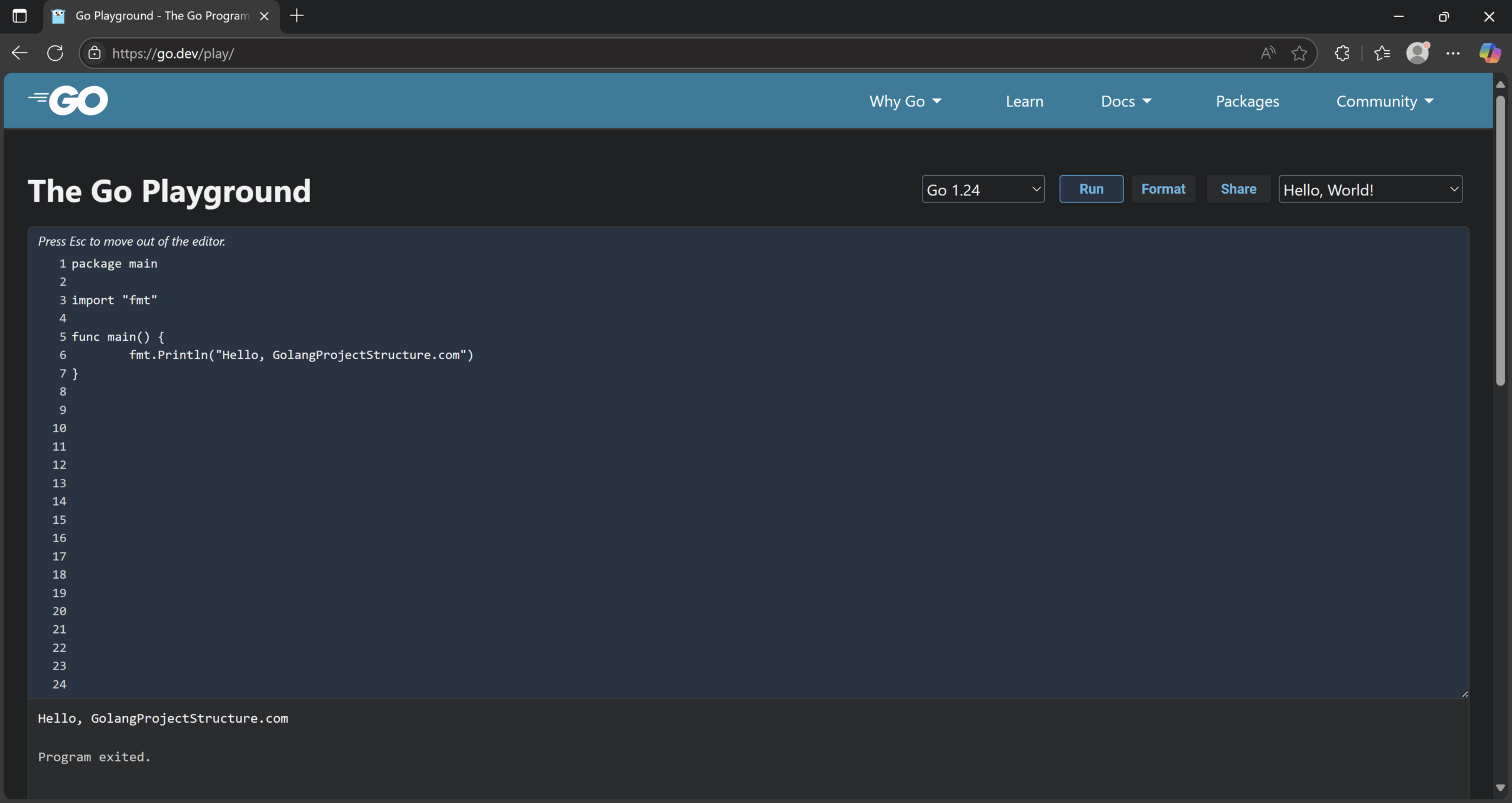
The Go Playground is available at the following URL: https://go.dev/play/
Because it is a browser-based tool, the Playground requires no downloads.
Users can simply navigate to the URL above using any modern web browser and start writing code straightaway.
This accessibility ensures that the Playground can be reached from virtually any device connected to the internet, whether that be a desktop computer, laptop, tablet or smartphone.
If you forget the URL, just type the words "go playground" into a search engine, and the correct website should be returned as one of the top results.
Many tutorials, documentation pages and community-supported forums include direct links to code examples that are hosted on the Go Playground.
This common point of access not only simplifies the sharing of code but also actively encourages collaboration and discussion, enabling developers worldwide to learn from one another’s examples within a shared interactive space.
How Does the Go Playground Work?
The Go Playground functions within a secure, tightly controlled sandboxed environment, meticulously designed to ensure that all code execution is both safe and predictable.
By isolating user code from the host system, the Playground maintains a robust level of security while offering a reliable and consistent development experience.
Underlying Architecture
When code is submitted via the Playground, it is transmitted to backend servers maintained by the Go development team.
These servers are responsible for compiling and executing the code, and the resulting output is relayed back to the user through the web interface.
This process is seamless and requires no local computation beyond the use of a standard web browser.
Secure Execution Model
The Go Playground supports a substantial subset of the standard Go library, yet it imposes restrictions on certain packages, particularly those requiring system calls.
This is a deliberate security measure designed to maintain the integrity of the sandboxed environment.
Code execution follows a deterministic model, ensuring that identical input consistently yields the same output, a feature that significantly enhances caching and reproducibility.
Interestingly, the Playground sets the current time to 2009-11-10 23:00:00 UTC. This choice is deliberate and aids in deterministic output generation, allowing efficient caching and comparison of results.
Furthermore, for security reasons, both network and filesystem access are entirely disabled, thereby preventing unauthorised interactions with external systems.
To curtail resource exploitation, execution time is rigorously constrained, and CPU and memory allocations are tightly controlled, ensuring fair usage across all users of the Playground.
Is There a Better Version of the Go Playground?
The official Go Playground is a widely used and well-maintained tool, yet it is not the only online environment available for writing and executing Go code.
One notable alternative is GoPlay, a third-party Go playground that extends the functionality of the official version with a range of enhanced features.
How Does GoPlay Improve Upon the Official Playground?
Support for External Dependencies
One of the most significant limitations of the official Go Playground is its confinement to the standard library, which prevents developers from testing code that relies on third-party packages.
GoPlay overcomes this by allowing users to import external modules via support for Go modules, making it a far more versatile option for real-world experimentation.
Advanced Code Formatting and Linting
While the official Playground does provide basic formatting via gofmt, GoPlay goes further by integrating linters and additional formatting options, helping developers adhere to best coding practices and maintain cleaner code.
An Improved User Interface
GoPlay also offers an enhanced coding experience with a more sophisticated editor that includes features such as syntax highlighting, autocompletion and bracket matching.
These small refinements can significantly improve productivity, particularly for those writing larger code snippets.
Execution Tracing and Debugging Tools
Yet another limitation of the standard Playground is its lack of execution profiling and tracing capabilities.
GoPlay introduces advanced debugging features, including runtime analysis and performance insights, allowing developers to better understand the behaviour of their code.
Support for Custom Go Versions
Since Go evolves rapidly, developers often want to experiment with beta releases or older versions of the language.
GoPlay accommodates this by enabling users to select from multiple Go versions, making it ideal for compatibility testing or exploring new features prior to their general adoption.
Collaboration and Code Sharing
While the official Go Playground does allow users to generate shareable URLs, GoPlay refines this experience with improved code-sharing options.
These include GitHub integration, embedding functionality and even real-time collaborative editing, making it a more compelling platform for pair programming, team-based development, and instructional us
How Can I Compare GoPlay With the Original Go Playground?
The table below summarises the most important differences between the official Go Playground and GoPlay, to help you select between them:
| Feature | Official Go Playground | GoPlay (Third-Party Alternative) |
|---|---|---|
| Access to Standard Library | ✅ Access provided | ✅ Access provided |
| Support for External Packages | ❌ Not supported | ✅ Supported via Go modules |
| Code Formatting | ✅ Basic formatting via gofmt | ✅ Advanced formatting with linting tools |
| Editor Features | ⚠️ Minimal editor (basic text input only) | ✅ Enhanced editor: syntax highlighting, autocompletion, bracket matching |
| Runtime Debugging Tools | ❌ Not available | ✅ Includes execution tracing and debugging support |
| Time Handling | 🔁 Time fixed to 2009-11-10 23:00:00 UTC for determinism | ⏱ Realistic time support (varies by configuration) |
| Network and Filesystem Access | ❌ Fully restricted | ⚠️ Limited or configurable (depends on GoPlay’s sandbox model) |
| Multiple Go Versions | ❌ Only latest stable version | ✅ Selectable Go versions (including betas and past releases) |
| Collaboration Features | ✅ Shareable URLs only | ✅ GitHub integration, embedding, real-time collaborative editing |
| Use Case Suitability | ✅ Ideal for learning and quick experiments | ✅ Better for real-world testing, team collaboration, and debugging |