I know it sounds like a funky dance move, but the Knuth shuffle is actually an elegant method for randomly rearranging the elements in an array — or, as we Gophers tend to prefer, a slice.

The algorithm is very easy to understand and implement, which means that you should be able to use it in your own code whenever you need to shuffle the elements of a slice or array.

Who Was Donald Knuth?

The Knuth shuffle is named after Donald Knuth, a man whom every serious programmer should be aware of, so let’s introduce him by giving a brief overview of some important aspects of his life and work.

Donald Knuth was born in 1938, and he would soon become a world-famous academic in the nascent field of computer science. However, he began his studies by concentrating on the interrelated fields of mathematics and physics.

However, even in the 1950s, when he was working towards his undergraduate degree, he had an interest in computing, and he spent time working on his own assembler and compiler programs for the college’s mainframe computer.

He went on to join the faculty at both the California Institute of Technology and Stanford University, where he did a great deal of ground-breaking work.

For example, Donald Knuth is responsible for inventing the TeX typesetting system, which provides an ingenious way to publish documents containing complex mathematical formulae.

You might have seen his multi-volume magnum opus titled The Art of Computer Programming.

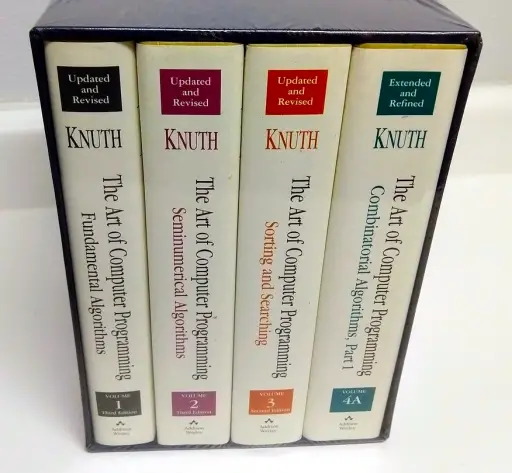
That series of books is one of the most important academic works ever written on the design, implementation and analysis of algorithms.

Knuth’s writing style is clear and precise. However, given his background, it is unsurprising that he places a very strong emphasis on the use of formal mathematics to prove the correctness of the algorithms that he describes.

That relentless focus on intellectual rigour is what makes his text so appealing to academics and top-level coders alike — yet it can also intimidate those who don’t have such a highly honed interest in abstract thinking for its own sake (so it is no insult to Knuth to admit that a less imposing work should probably be chosen as a first introductory guide to the subject of algorithms).

Bill Gates, who needs little introduction as one of the most famous tech entrepreneurs in the world, thanks to his co-founding of Microsoft, once said:

If you think you’re a really good programmer, read The Art of Computer Programming. You should definitely send me a résumé if you can read the whole thing.

It was in Volume Two of The Art of Computer Programming that the Knuth shuffle was described and discussed [under the rather unmemorable heading “Algorithm P (Shuffling)”].

This shuffling technique came to be named after Donald Knuth since it was popularized by him in that book, but the algorithm had originally appeared in an earlier article by Richard Durstenfeld, who was a much less famous mathematician working at the General Atomics corporation.

Even this algorithm, however, was a modified version of an earlier algorithm called the Fisher–Yates shuffle, named after Ronald Fisher and Frank Yates, who were both highly accomplished British statisticians.

In the following sections of this blog post, we’ll look at these two shuffling algorithms in more detail — the Knuth shuffle and the original Fisher–Yates shuffle — including implementations of each algorithm in code that’s written in the Go programming language.

Creating a Slice

Let’s begin by initializing a slice and filling it with numbers, so we have something to work with when we begin implementing the shuffle:

numbers.go

package main

import "fmt"

const numbersCount = 20

var numbers []int

func init() {
	numbers = make([]int, numbersCount)

	for i := range numbers {
		numbers[i] = i + 1
	}

	fmt.Println(numbers)
}

There isn’t a great deal to talk about here, since the code is pretty self-explanatory.

However, you can see that we use the built-in make function in order to initialize the numbers slice with a length of 20, ensuring that sufficient memory is allocated.

Then we simply iterate through the slice, setting each value to a number equivalent to one greater than the index (so that the value at index 0 is 1 and the value at index 13 is 14 etc.).

This means that while the slice’s indices run from zero to nineteen inclusive, the values go from one to twenty inclusive.

We can see this if we run the code above, which will produce the following output:

[1 2 3 4 5 6 7 8 9 10 11 12 13 14 15 16 17 18 19 20]

The slice has been populated with the twenty values that we had expected.

Performing the Knuth Shuffle

The code below shows how the Knuth shuffle is actually implemented, using the numbers slice that we initialized in the previous example:

main.go

package main

func init() {
	rand.Seed(time.Now().UnixNano())
}

func main() {
	for i := len(numbers) - 1; i >= 1; i-- {
		j := rand.Intn(i + 1)

		numbers[i], numbers[j] = numbers[j], numbers[i]
	}

	fmt.Println(numbers)
}

We begin by seeding Go’s random-number generator with a timestamp, in order to ensure that we don’t get the same set of random numbers every time that we run this program.

Then we iterate through the numbers slice that we created in the earlier example. We iterate in reverse order, from the last index all the way down to the second index (not the first — but remember that the second index has a value of 1 in Go, since our programming language uses zero-based indices).

Then in each iteration of the for loop, we declare a variable j and assign to it a random number between 0 and i inclusive (the rand.Intn function takes i + 1 as its argument because it works with an exclusive upper bound).

We simply swap the value at index i with the value at index j. Note that we are able to use an idiomatic one-liner to do this in Go, whereas other C-based languages would require the use of an additional temporary variable when performing the swap.

Finally, once the algorithm is complete, we print out the shuffled slice, in order to demonstrate that the elements now have a different ordering to the one that was printed when we first initialized the slice.

If you run this program multiple times, it should give a different ordering every time (unless you’re lucky enough to randomly select the same ordering two times in a row, which is so exceptionally unlikely with a slice of this size that I can’t imagine it actually happening, assuming that your code has been written correctly).

Comparing the Original Fisher–Yates Algorithm

Now we’ve seen the shuffle algorithm that was popularized by Donald Knuth, let’s take a moment to look at the original shuffling algorithm devised by Fisher–Yates:

main.go

package main

func init() {
	rand.Seed(time.Now().UnixNano())
}

func main() {
	unseenIndices := make([]int, len(numbers))

	for i := 0; i < len(numbers)-1; i++ {
		unseenIndices[i] = i
	}

	shuffledNumbers := make([]int, 0, len(numbers))

	for len(shuffledNumbers) < len(numbers) {
		index := -1

		for index == -1 {
			index = unseenIndices[rand.Intn(len(unseenIndices))]
		}

		unseenIndices[index] = -1

		value := numbers[index]

		shuffledNumbers = append(shuffledNumbers, value)
	}

	fmt.Println(shuffledNumbers)
}

Within the main function, we begin by creating another slice that will be used to keep track of which indices of the numbers slice we’ve already handled.

Then we create yet another slice that will hold the shuffled numbers, since this algorithm does not shuffle the numbers in place, but rather moves them into a new slice.

We give the shuffledNumbers slice the same capacity as the numbers slice, but its length starts at zero and we iterate until its length is equivalent to that of the original numbers slice.

Within each iteration, we choose a random index from the unseenIndices slice. However, once we’ve seen an index, we set the value at that index within the unseenIndices slice to -1, in order to signify that we should no longer choose that index, so we continue choosing a random index until the value at it no longer equals -1.

Then we simply append the value at the chosen index in our numbers slice to our shuffledNumbers slice, gradually building up its size.

Just remember that this algorithm is like picking a card at random from a deck of cards — ignoring the cards that have already been picked — and adding another card identical to the one picked to a new deck until the size of the new deck is the same as the old one.

Indeed, the algorithm was originally published in 1938 and was intended to be applied manually to datasets by statisticians and other scientists with the help of a pencil and paper. It was only later that the algorithm was converted to run on a computer.

Why Is the Knuth Shuffle Faster Than the Fisher–Yates Shuffle?

When thinking about performance, the most obvious thing to note is that the algorithm described in Donald Knuth’s The Art of Computer Programming book shuffles the original slice, whereas the Fisher-Yates algorithm requires an additional slice for its output. Naturally, this means that the Knuth shuffle uses less memory.

However, more important is the fact that the Fisher-Yates algorithm uses a nested loop in order to skip indices that have already been seen, whereas the Knuth algorithm simply iterates through each element in the original slice only once. This means that much less processing power is used when shuffling large slices.

Using Big O Notation, the Fisher-Yates shuffling algorithm has a time complexity of O(n²), whereas the Knuth algorithm has a time complexity of O(n) — which, of course, makes it much faster as n increases.

In other words, the Knuth shuffle runs in linear time, whereas the Fisher-Yates shuffle runs in quadratic time.