It’s reasonable to look at a picture and to wonder how it might look if it were distilled down into a single colour, which somehow still encapsulates a sense of the original.

In this post, we will look at various methods that can be used to calculate the average colour of an image in Go, taking into account all of the different colours that are used in the image.

Prerequisite Knowledge

This post is designed to be accessible for relative beginners, however, if you’re not familiar with loading images and manipulating pixels in Go, I suggest that you first read my article about converting full-colour images into greyscale, since that goes over some of the basic concepts that we’ll be using to calculate the average colour of an image.

If you don’t want to do that, then don’t worry, because you should still be able to continue reading this post and follow along with everything easily enough: just be sure to look up any code that you don’t understand, especially in the first examples.

The Artwork That We’ll Be Using in Our Example Code

I’m going to use the same image in all of the example code below. The image I have chosen is a scan of an original painting by Berthe Morisot (1841–1895), who was a female French Impressionist artist. She had her artwork exhibited alongside perhaps now more famous contemporaries such as Claude Monet and Paul Cézanne.

The painting shows a young girl sitting alongside a small dog. The girl is holding the dog’s paw in her hand as it looks into her eyes. It is a tender scene of friendship and affection between a child and her beloved pet.

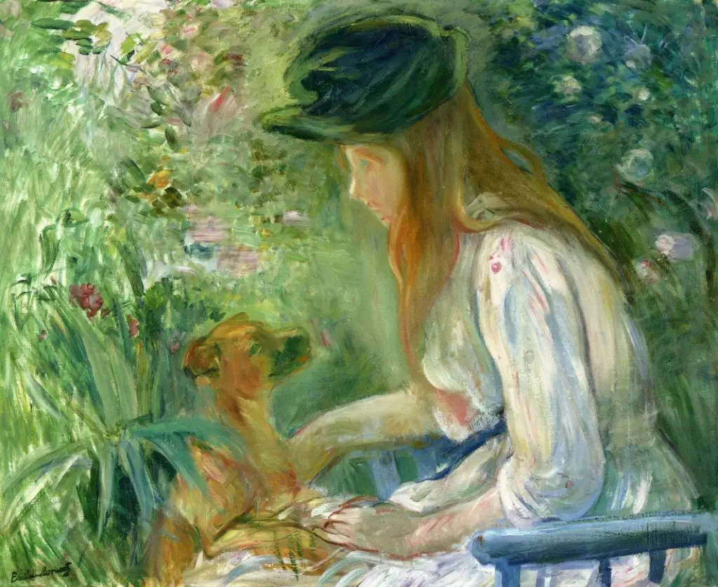
There are lots of bright colours in the image, from the white of the girl’s dress to the brown of her hair and the dog’s fur. However, the majority of the background is made up of shades of green, since the girl is sitting in a garden surrounded by plants and foliage. It appears that there is a pond in the top-right corner of the painting, which is dominated by a blue-green tint.

We can, therefore, expect the average colour of the image to be relatively greenish. This initial assumption allows us to check the accuracy of our algorithms, since if we run some code that calculates the average colour to be a shade of red, for example, we know that we must have done something wrong, because there’s so little red in the original image that it simply can’t be the average colour.

Adding All the Pixels to Get a Mean Value

When most people want an average, they’re usually thinking about the mean value, which is really easy to calculate. For example, if we want to find the mean of a list of numbers, we can simply add them all up to produce a total, and then divide that total by the amount of numbers we had in our initial list.

We can, of course, do this in Go very easily:

package main

import (
	"fmt"
)

func main() {
	numbers := []float64{5, 4, 3, 6, 8, 10, 7, 5, 3, 6, 8, 1, 8}

	var total float64
	for _, n := range numbers {
		total += n
	}

	meanAverage := total / float64(len(numbers))

	fmt.Printf("Our average number is "%f".n", meanAverage)
}

If you run the example above, you should find that average value of all the numbers in the slice we defined is 5.54 (once rounded to two decimal places).

We can now apply this principle to our image, creating a mean value from all of the colours that it contains:

package main

import (
	"fmt"
	"image"
	"image/color"
	_ "image/jpeg"
	"log"
	"math"
	"os"
)

func main() {
	file, err := os.Open("girl-with-a-dog-by-berthe-morisot.jpg")
	if err != nil {
		log.Fatalln(err)
	}
	defer file.Close()

	img, _, err := image.Decode(file)
	if err != nil {
		log.Fatalln(err)
	}

	imgSize := img.Bounds().Size()

	var redSum float64
	var greenSum float64
	var blueSum float64

	for x := 0; x < imgSize.X; x++ {
		for y := 0; y < imgSize.Y; y++ {
			pixel := img.At(x, y)
			col := color.RGBAModel.Convert(pixel).(color.RGBA)

			redSum += float64(col.R)
			greenSum += float64(col.G)
			blueSum += float64(col.B)
		}
	}

	imgArea := float64(imgSize.X * imgSize.Y)

	redAverage := math.Round(redSum / imgArea)
	greenAverage := math.Round(greenSum / imgArea)
	blueAverage := math.Round(blueSum / imgArea)

	fmt.Printf(
		"Average colour: rgb(%.0f, %.0f, %.0f)n",
		redAverage,
		greenAverage,
		blueAverage,
	)
}

You can see above how we simply iterate through each pixel of the image, adding the red, green and blue values for each pixel to three variables that will contain the totals. Then we divide each of the totals by the number of pixels in the entire image, which can be calculated simply by multiplying the image’s height by its width.

This gives us the average red, green and blue values, which are then simply printed out to the screen.

We initially convert the RGB values to floating-point numbers, so that when we do the division on each of the totals, the result won’t be rounded down, as it would have been if we’d used some kind of integer.

It doesn’t make sense to have a fractional part of a colour, however, so we round the averages either up or down (depending on which is the nearest whole number) using the math.Round function from the standard library.

We could, at this point, have converted the final averages to uint8 values, which is what I would have done if I’d been intending to use the averages in some other code. But since we’re just outputting them to the screen with the fmt.Printf function, I used the "%.0f" format parameter to have each floating-point number be printed without a decimal point.

So when I run the code in the example above, I get the following output:

Average colour: rgb(119, 138, 99)

Viewing the Average Colour Using a Simple Webpage

If you want a more visual representation, you can create a very simple HTML page with the RGB colour set to fill the background, as shown below. When you open it in your web browser, you’ll be able to see the average colour that we’ve calculated.

<!DOCTYPE html>
<html>
	<head>
		<title>The Average Color (Mean)</title>
	</head>
	<body style="background-color: rgb(119, 138, 99);"></body>
</html>

The result should look something like this:

Given how much green is in the original image (with all the garden plants and pond-lilies behind the girl and her dog), I think it’s fair to say that our average colour seems pretty representative.

Experiment With My Code for Yourself

I encourage you to copy-and-paste the example code we looked at above and run it on your own machine with one of your own images, so you can see how the average changes when given different input.

Whenever we work on example projects like this, don’t just take my word for anything: always experiment and play with the code yourself.

There may be cases when you discover a weird bug that only occurs in certain circumstances — I hope you don’t, but tell me if you do! — or you may simply find yourself adding an interesting new feature that I hadn’t thought about.

In any case, you’ll always learn more by actively engaging with my code than just by skim-reading through it. The core concepts and syntax will stick in your mind better.

Taking a Short Detour: Calculating a Delta From the Average

This section isn’t strictly necessary, so feel free to skip it and move onto the next one, if you just want to focus on the important stuff. I just thought it would be interesting to see how “average” the average colour actually is.

That’s not the best way to put it, I know, but what I mean is how well the average colour represents the original image. For example, the average colour of an image that contains a wide range of different colours will be less representative than the average colour of an image that contains a smaller number of similar colours.

The average value will be farther away from the colour of most pixels in a multicolored image and closer to the colour of most pixels in a more similarly shaded image. Let’s have a look at some code, and that should help to explain the general concept that I’m trying to get across:

package main

import (
	"fmt"
	"image"
	"image/color"
	_ "image/png"
	"log"
	"math"
	"os"
)

type calculateMeanAverageColourWithDeltaResult struct {
	averageRed   uint8
	averageGreen uint8
	averageBlue  uint8

	deltaRed   uint8
	deltaGreen uint8
	deltaBlue  uint8
}

func calculateMeanAverageColourWithDelta(img image.Image) (result calculateMeanAverageColourWithDeltaResult) {
	imgSize := img.Bounds().Size()

	var redSum float64
	var greenSum float64
	var blueSum float64

	for x := 0; x <= imgSize.X; x++ {
		for y := 0; y <= imgSize.Y; y++ {
			pixel := img.At(x, y)
			col := color.RGBAModel.Convert(pixel).(color.RGBA)

			redSum += float64(col.R)
			greenSum += float64(col.G)
			blueSum += float64(col.B)
		}
	}

	imgArea := float64(imgSize.X * imgSize.Y)

	result.averageRed = uint8(math.Round(redSum / imgArea))
	result.averageGreen = uint8(math.Round(greenSum / imgArea))
	result.averageBlue = uint8(math.Round(blueSum / imgArea))

	redSum = 0
	greenSum = 0
	blueSum = 0

	for x := 0; x < imgSize.X; x++ {
		for y := 0; y < imgSize.Y; y++ {
			pixel := img.At(x, y)
			col := color.RGBAModel.Convert(pixel).(color.RGBA)

			redSum += math.Abs(float64(result.averageRed) - float64(col.R))
			greenSum += math.Abs(float64(result.averageGreen) - float64(col.G))
			blueSum += math.Abs(float64(result.averageBlue) - float64(col.B))
		}
	}

	result.deltaRed = uint8(math.Round(redSum / imgArea))
	result.deltaGreen = uint8(math.Round(greenSum / imgArea))
	result.deltaBlue = uint8(math.Round(blueSum / imgArea))

	return
}

func main() {
	file, err := os.Open("chessboard-with-black-and-white-alternating-squares.png")
	if err != nil {
		log.Fatalln(err)
	}
	defer file.Close()

	img, _, err := image.Decode(file)
	if err != nil {
		log.Fatalln(err)
	}

	result := calculateMeanAverageColourWithDelta(img)

	fmt.Printf(
		"Average colour: rgb(%d, %d, %d)n",
		result.averageRed,
		result.averageGreen,
		result.averageBlue,
	)

	fmt.Printf(
		"Delta:          rba(%d, %d, %d)n",
		result.deltaRed,
		result.deltaGreen,
		result.deltaBlue,
	)
}

I have created a struct to hold the return values of the calculateMeanAverageColourWithDeltaResult function, simply to keep things tidy, since we’re going to be returning six different integers: one for each of the three RGB values that make up the average colour that we already calculated in the previous section and another three RGB values that make up the average delta.

You can see that we use a second loop to help us calculate the average delta by adding up the absolute distance (using the math.Abs function) between the colour of each pixel and the average colour and then dividing by the the total number of pixels. So we’re calculating another mean value, just as we did earlier.

When I run this code, I get the following output:

Average colour: rgb(119, 139, 99)
Delta:   rgb(45, 39, 40)

We already know how to think about the average colour, but how do we interpret the delta? It may be useful to think about the maximum and minimum possible values that the delta can have, so we can judge whether our result is particularly low or high.

Let’s consider a hypothetical image that is made up of only one colour. It doesn’t matter what that colour happens to be: we know that the average colour will always be the same colour as entire image.

In that case, we can infer that the three delta values would all be zero, because that’s what they measure: how far away the average is from all of the colours that make up the whole image. There would be no distance between them, so the delta can only be three zeros.

Let’s use the following image, which is a block of solid purple, to test our intuition:

When we use this as the input to the code we wrote above, we get the following result, just as we had expected:

Average colour: rgb(128, 0, 128)
Delta:          rgb(0, 0, 0)

So that’s the minimum value we can possibly get as a delta. Now let’s think how about we can generate a delta: we want the maximum distance between our average colour and the other colours in the image.

If we have an image that is made up of an equal amount of white and black pixels, the average will be grey, but white and black are exact opposites on the colour spectrum, so they’re as far apart from each other as two different colours can possibly be. That must mean that they’re also as far apart from the average as it’s possibly be.

We can use the image of a chessboard that was generated as part of an example in a post that I wrote a few months ago, since it has 64 squares, 32 of which are coloured black and 32 of which are coloured white. So it fits the definition of an image with the same number of black and white pixels.

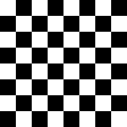
When we feed this image into our program, it produces the following result:

Average colour: rgb(128, 128, 128)
Delta:          rgb(128, 128, 128)

So whereas the each integer that makes up the average colour can have a value between zero and two hundred and fifty-six, each integer that makes up the average delta can have a value between zero and one hundred and twenty-eight.

So the delta that we got for our original image was closer to the minimum value than the maximum (because each integer was closer to 0 than 128). This implies that our image has a lot of colours that share a similar shade. We can see that this is true, because there’s clearly so much green in the original painting, but it’s nice to have it confirmed mathematically.

The concept of the delta is interesting, but we’re not going to use it in our subsequent code. However, you can calculate deltas for some of the functions that we’re going to write in the next sections, if you like.

Squaring the Colour Values

However, there is one small improvement we can make to the original calculateMeanAverageColour we created. The computer scientist Manohar Vanga wrote an interesting article a few years ago, in which he argued that we should be multiplying the value of each colour by itself (i.e. squaring it) before we calculate the sum. That is what we do in the code below:

package main

import (
	"fmt"
	"image"
	"image/color"
	_ "image/jpeg"
	"log"
	"math"
	"os"
)

func calculateMeanAverageColour(img image.Image, useSquaredAverage bool) (red, green, blue uint8) {
	imgSize := img.Bounds().Size()

	var redSum float64
	var greenSum float64
	var blueSum float64

	for x := 0; x < imgSize.X; x++ {
		for y := 0; y < imgSize.Y; y++ {
			pixel := img.At(x, y)
			col := color.RGBAModel.Convert(pixel).(color.RGBA)

			if useSquaredAverage {
				redSum += float64(col.R) * float64(col.R)
				greenSum += float64(col.G) * float64(col.G)
				blueSum += float64(col.B) * float64(col.B)
			} else {
				redSum += float64(col.R)
				greenSum += float64(col.G)
				blueSum += float64(col.B)
			}
		}
	}

	imgArea := float64(imgSize.X * imgSize.Y)

	if useSquaredAverage {
		red = uint8(math.Round(math.Sqrt(redSum / imgArea)))
		green = uint8(math.Round(math.Sqrt(greenSum / imgArea)))
		blue = uint8(math.Round(math.Sqrt(blueSum / imgArea)))
	} else {
		red = uint8(math.Round(redSum / imgArea))
		green = uint8(math.Round(greenSum / imgArea))
		blue = uint8(math.Round(blueSum / imgArea))
	}

	return
}

func main() {
	file, err := os.Open("girl-with-a-dog-by-berthe-morisot.jpg")
	if err != nil {
		log.Fatalln(err)
	}
	defer file.Close()

	img, _, err := image.Decode(file)
	if err != nil {
		log.Fatalln(err)
	}

	redAverage, greenAverage, blueAverage := calculateMeanAverageColour(img, true)

	fmt.Printf(
		"Average: rgb(%d, %d, %d)n",
		redAverage,
		greenAverage,
		blueAverage,
	)
}

So the major difference here, compared to our previous example, is that if useSquaredAverage is set to true, the variables used to sum up the three colour values are squared before they are added to the total. We could have used the math.Pow function from the Go standard library in order to perform the squaring calculation, but it’s easy enough in this case just to multiple the value by itself. If we had been raising

If we have squared the original values before adding them to the sum variables, we do, however, have to remember to take the square root of the mean values after dividing our sums by the total number of pixels. Since we use the math.Sqrt function, which returns a float64 type where the value is unlikely to be an integer, we have also used the math.Round function in order to ensure that each of our colour values only contains an integer between zero and two hundred and fifty-six.

You can see that the resulting colour (shown below) is very subtly brighter than the one that our previous code generated:

If you don’t believe me, create two webpages with each with the background set to a different one of the two colours and open them up in a browser side-by-side. The article by Manohar Vanga predicted that the squared average would be a lighter colour (because human vision works on a relative and somewhat logarithmic scale, which squaring the mean takes into account).

Calculating the Modal Average Colour

While the mean may be the most commonly used type of average, it’s certainly not the only one. Another kind of average that is useful when calculating an average colour is the mode. This type of average is not too difficult to understand, because the mode is simply the most commonly occurring value. Let’s take a look at a simple example with a list of numbers:

package main

import (
	"fmt"
)

func main() {
	numbers := []float64{5, 4, 3, 6, 8, 10, 7, 5, 3, 6, 8, 1, 6}

	counts := make(map[float64]int)
	for _, n := range numbers {
		counts[n]++
	}

	var highestCount int
	var highestCountNumber float64

	for n, i := range counts {
		if i > highestCount {
			highestCount = i
			highestCountNumber = n
		}
	}

	modeAverage := highestCountNumber

	fmt.Printf("Our modal average number is "%f".n", modeAverage)
}

If you run the code above, you will see that the modal average is six, because that number occurs three times in the original slice of numbers, whereas all of the other numbers in the slice occur less often. I think that’s pretty easy to understand, but don’t worry if you’re still a little uncertain about how the code actually works, because next we’ll apply the concept to getting the average colour in our image and then I’ll discuss exactly how everything fits together.

Here’s the new function:

package main

import (
	"fmt"
	"image"
	"image/color"
	_ "image/jpeg"
	"math"
	"os"
	"strconv"
	"strings"
)

func calculateModalAverageColour(
	img image.Image,
	useSquaredAverage bool,
) (red, green, blue uint8, err error) {
	imgSize := img.Bounds().Size()

	colourCounts := make(map[string]int)

	for x := 0; x < imgSize.X; x++ {
		for y := 0; y < imgSize.Y; y++ {
			pixel := img.At(x, y)
			col := color.RGBAModel.Convert(pixel).(color.RGBA)

			colourKey := fmt.Sprintf("%d:%d:%d", col.R, col.G, col.B)

			colourCounts[colourKey]++
		}
	}

	var modalColours []string
	var modalCount int

	for colour, count := range colourCounts {
		if count > modalCount {
			modalCount = count

			modalColours = modalColours[:0]
		}

		if count >= modalCount {
			modalColours = append(modalColours, colour)
		}
	}

	var redTotal float64
	var greenTotal float64
	var blueTotal float64

	for _, m := range modalColours {
		modalColourSplit := strings.Split(m, ":")
		modalColourUint64 := make([]uint64, 3)

		for i, c := range modalColourSplit {
			modalColourUint64[i], err = strconv.ParseUint(c, 10, 0)
			if err != nil {
				return
			}
		}

		if useSquaredAverage {
			redTotal += float64(modalColourUint64[0]) * float64(modalColourUint64[0])
			greenTotal += float64(modalColourUint64[1]) * float64(modalColourUint64[1])
			blueTotal += float64(modalColourUint64[2]) * float64(modalColourUint64[2])
		} else {
			redTotal += float64(modalColourUint64[0])
			greenTotal += float64(modalColourUint64[1])
			blueTotal += float64(modalColourUint64[2])
		}
	}

	modalColoursTotal := float64(len(modalColours))

	if useSquaredAverage {
		red = uint8(math.Round(math.Sqrt(redTotal / modalColoursTotal)))
		green = uint8(math.Round(math.Sqrt(greenTotal / modalColoursTotal)))
		blue = uint8(math.Round(math.Sqrt(blueTotal / modalColoursTotal)))
	} else {
		red = uint8(math.Round(redTotal / modalColoursTotal))
		green = uint8(math.Round(greenTotal / modalColoursTotal))
		blue = uint8(math.Round(blueTotal / modalColoursTotal))
	}

	return
}

As you can see above, the code in the calculateModalAverageColour function is significantly more complex — or, at least, it extends over many more lines — than the code in the calculateMeanAverageColour that we previously defined.

This is because we now have three loops, instead of just one, inside the function that calculates a modal-average colour.

The first loop simply iterates through each of the pixels and increments a counter for each colour, so we can see how many times a certain colour appears, and reappears, in the image. In order to make this easier, we create a key, which is a string type that incorporates all three of the RGB values.

The second loop iterates through our counter, finding the colour that appears the most number of times. We add it to a slice, which allows us to add more than one colour, if we find that there are multiple colours that all appear exactly at exactly the highest frequency.

Finally, in the third loop, we use the mean-averaging code that we saw in our first example. If our modalColours slice only contained one colour, we could simply have returned that value, since that is the single most frequently occurring colour in the image.

However, if modalColours contains more than one colour, then we return the mean value of the multiple modes (by adding them all up and dividing by the total number of modes), in order to ensure that we only ever return a single colour.

I have chosen to perform the final mean-averaging calculation even if there is only one mode, since it makes the code slightly easier to write: any average of a single value will always be identical to the value itself. If you’re concerned about the computer doing a very small amount of unnecessary work, you could, however, modify the function to include an if-clause that returns early whenever there is no more than one mode.

This shade of green is noticeably lighter than the two mean-average colours we calculated. This is because there are simply so many light-green pixels in the image. Look at the area to the left of the girl’s face in the original painting, and you will see shades of green that are not dissimilar to the modal-average colour.

Getting the Average Colour Within a Rectangular Segment of the Image

Now that we understand how to produce two slightly different values (using the mean and the mode) for the average colour of an image, let’s try something else. In the image below, I’ve drawn a red rectangle around the dog’s head, as you can see:

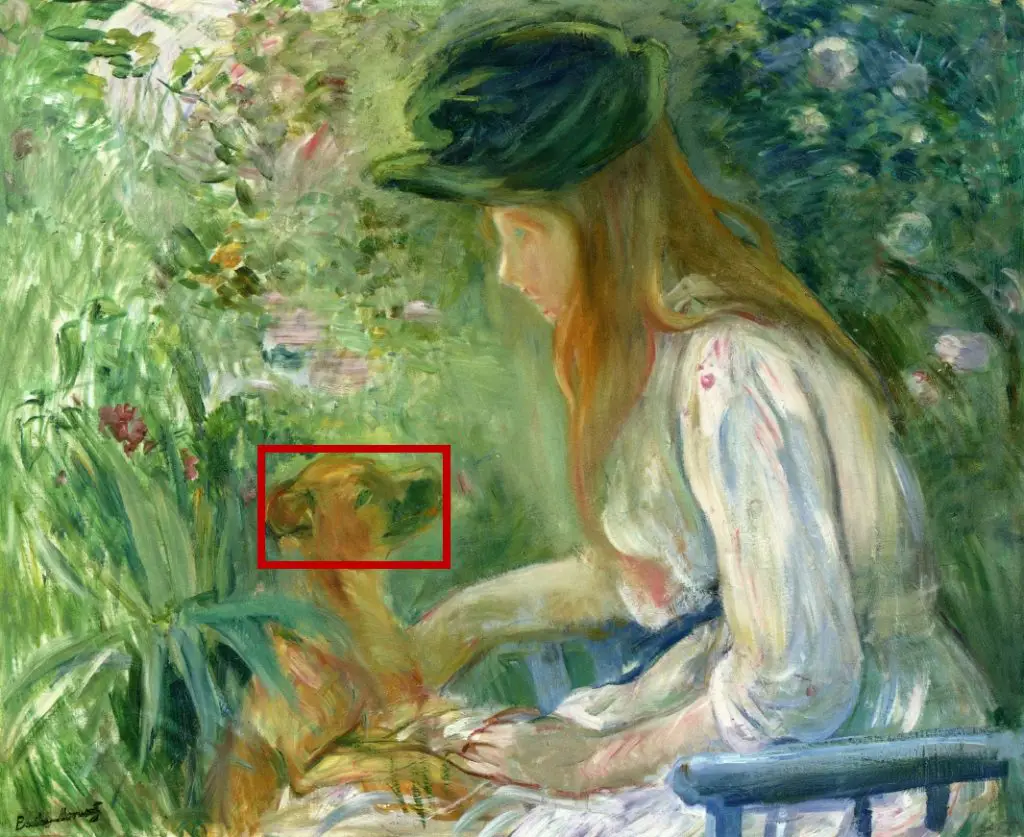
In the code that we write in this section, we’re going to use the original image but only get the average colour of the pixels within that smaller area where the red rectangle is. So, in effect, we’re just getting the average of the smaller image below, even though we never actually create this cropped image:

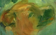
This can be useful if we simply want to extract the colour of a particular section of an image that we find attractive. The example below shows how we can implement this in Go code:

package main

import (
	"fmt"
	"image"
	"image/color"
	_ "image/jpeg"
	"log"
	"math"
	"os"
)

func calculateMeanAverageColourWithRect(
	img image.Image,
	rect image.Rectangle,
	useSquaredAverage bool,
) (red, green, blue uint8) {
	var redSum float64
	var greenSum float64
	var blueSum float64

	for x := rect.Min.X; x <= rect.Max.X; x++ {
		for y := rect.Min.Y; y <= rect.Max.Y; y++ {
			pixel := img.At(x, y)
			col := color.RGBAModel.Convert(pixel).(color.RGBA)

			if useSquaredAverage {
				redSum += float64(col.R) * float64(col.R)
				greenSum += float64(col.G) * float64(col.G)
				blueSum += float64(col.B) * float64(col.B)
			} else {
				redSum += float64(col.R)
				greenSum += float64(col.G)
				blueSum += float64(col.B)
			}
		}
	}

	rectArea := float64((rect.Dx() + 1) * (rect.Dy() + 1))

	if useSquaredAverage {
		red = uint8(math.Round(math.Sqrt(redSum / rectArea)))
		green = uint8(math.Round(math.Sqrt(greenSum / rectArea)))
		blue = uint8(math.Round(math.Sqrt(blueSum / rectArea)))
	} else {
		red = uint8(math.Round(redSum / rectArea))
		green = uint8(math.Round(greenSum / rectArea))
		blue = uint8(math.Round(blueSum / rectArea))
	}

	return
}

func main() {
	file, err := os.Open("girl-with-a-dog-by-berthe-morisot.jpg")
	if err != nil {
		log.Fatalln(err)
	}
	defer file.Close()

	img, _, err := image.Decode(file)
	if err != nil {
		log.Fatalln(err)
	}

	rect := image.Rect(
		272, 467,
		465, 588,
	)

	redAverage, greenAverage, blueAverage := calculateMeanAverageColourWithRect(img, rect, true)

	fmt.Printf(
		"Average: rgb(%d, %d, %d)n",
		redAverage,
		greenAverage,
		blueAverage,
	)
}

Much of the code in the calculateMeanAverageColourWithRect function is the same as we previously saw in the calculateMeanAverageColour function. The major difference is that it now takes an image.Rectangle parameter, which specifies the area in the image within which the average colour should be calculated.

Instead of iterating from zero on the x and y dimensions and ending at the width and height of the image, we now begin at the left-most and top-most points of the rectangle and stop at the right-most and bottom-most points.

The rect.Dx function calculates the width of the rectangle (literally, the delta, or difference, between the maximum x point and the minimum one). Likewise, the rect.Dy function calculates the height of the rectangle. So we can multiple these together to produce the total area of all the pixels within the rectangle.

I added one to the result of the rect.Dx and rect.Dy functions, because the Go standard library assumes that we don’t include the rect.Max.X and rect.Max.Y values in our iteration (i.e. by using the less than symbol in the loop conditions, rather than the less than or equal to symbol), but I chose to include them, because that made more sense to me, based on an inclusive definition of a maximum value.

The image.Rect function takes the coordinates of the two points that define our rectangle: the one in the top-left corner and the one in the bottom-right corner. It returns an image.Rectangle struct that we then pass to our function that calculates the mean-average colour within those given bounds.

The colour above is darker than any of the average colours that we’ve previously found. It is somewhere between brown and green. This is, of course, exactly what we’d expect since the dog’s fur is brown and the background foliage is green.

Calculating the Average of Multiple Areas in the Image

Now that we know how to produce the average colour for a specific rectangle-bounded area within an image, let’s build on that knowledge to create a function that can produce the average colour for all the pixels in an image that are within many different rectangles.

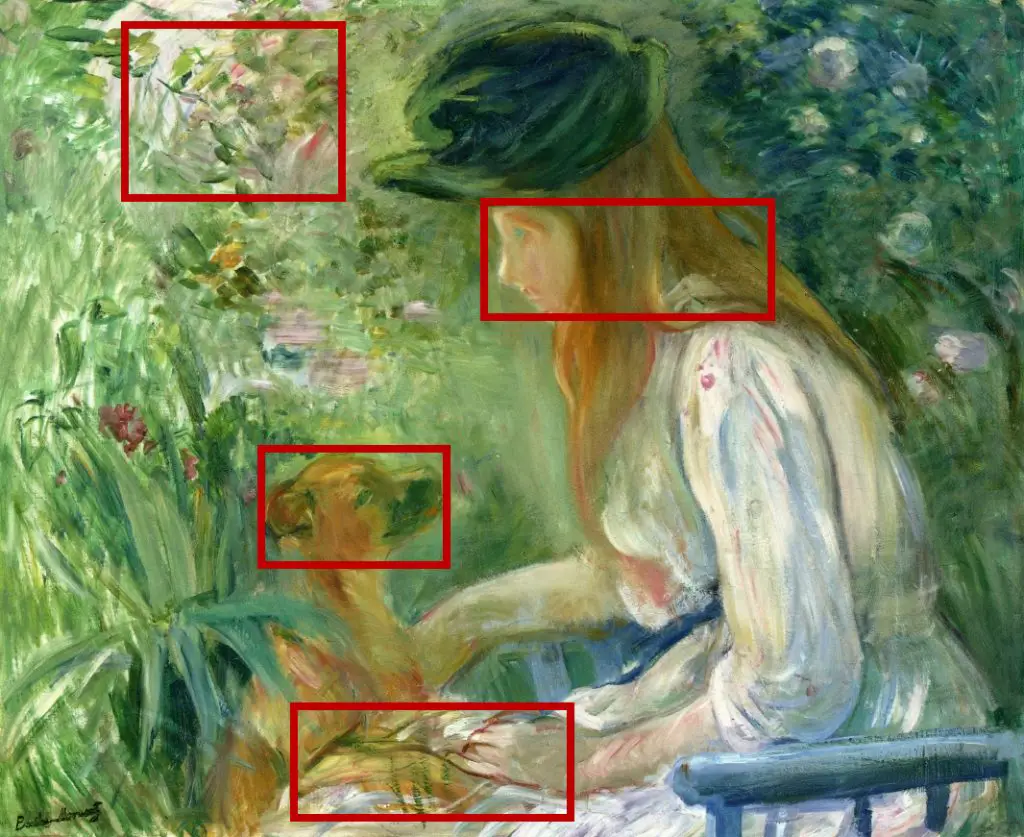
As you can see above, I’ve now selected four different areas of interest, where the eyes of the viewer may naturally be drawn as they look at the painting, while excluding much of the less interesting greenery in the background. We’re still including the dog’s head, as in the previous example, but now we’re also including the girl’s head, the dog’s paw as it holds the girl’s hand and a squarish patch of white and pink flowers.

The code below finds the average colour from the four rectangular areas we have defined:

package main

import (
	"fmt"
	"image"
	"image/color"
	_ "image/jpeg"
	"log"
	"math"
	"os"
)

func calculateMeanAverageColourWithMultipleRects(
	img image.Image,
	rects []image.Rectangle,
	useSquaredAverage bool,
) (red, green, blue uint8) {
	var redSum float64
	var greenSum float64
	var blueSum float64

	for _, r := range rects {
		for x := r.Min.X; x <= r.Max.X; x++ {
			for y := r.Min.Y; y <= r.Max.Y; y++ {
				pixel := img.At(x, y)
				col := color.RGBAModel.Convert(pixel).(color.RGBA)

				if useSquaredAverage {
					redSum += float64(col.R) * float64(col.R)
					greenSum += float64(col.G) * float64(col.G)
					blueSum += float64(col.B) * float64(col.B)
				} else {
					redSum += float64(col.R)
					greenSum += float64(col.G)
					blueSum += float64(col.B)
				}
			}
		}
	}

	var rectsArea float64

	for _, r := range rects {
		rectsArea += float64((r.Dx() + 1) * (r.Dy() + 1))
	}

	if useSquaredAverage {
		red = uint8(math.Round(math.Sqrt(redSum / rectsArea)))
		green = uint8(math.Round(math.Sqrt(greenSum / rectsArea)))
		blue = uint8(math.Round(math.Sqrt(blueSum / rectsArea)))
	} else {
		red = uint8(math.Round(redSum / rectsArea))
		green = uint8(math.Round(greenSum / rectsArea))
		blue = uint8(math.Round(blueSum / rectsArea))
	}

	return
}

func main() {
	file, err := os.Open("girl-with-a-dog-by-berthe-morisot.jpg")
	if err != nil {
		log.Fatalln(err)
	}
	defer file.Close()

	img, _, err := image.Decode(file)
	if err != nil {
		log.Fatalln(err)
	}

	rects := []image.Rectangle{
		image.Rect(272, 467, 465, 588), // dog's face
		image.Rect(504, 210, 803, 330), // girl's face
		image.Rect(306, 735, 594, 851), // dog's paw and girl's hand
		image.Rect(130, 26, 356, 206),  // floral patch
	}

	redAverage, greenAverage, blueAverage := calculateMeanAverageColourWithMultipleRects(img, rects, true)

	fmt.Printf(
		"Average: rgb(%d, %d, %d)n",
		redAverage,
		greenAverage,
		blueAverage,
	)
}

There isn’t too much to say about this code example, as so much is similar to what we saw before. Note, however, that we now have nested loops that are three levels deep. The inner two loops iterate through the pixels in the x and y directions, as before, but the outer loop now iterates through the different rectangles that we have passed through the function.

We ultimately produce a single average colour that takes into account all of the areas within our rectangles without being influenced by any of the pixels outside those areas.

It is necessary that none of the rectangles is overlapping with any of the others, since we’d end up counting the same pixel more than once, skewing our average. We could, if we were so inclined, write code that would replace any overlapping rectangles with ones that cover all the same areas but don’t overlap, in order to ensure that the function will still work properly, even if someone does accidentally call it with overlapping rectangles. But I’ll leave that as an exercise for you: if you want a little challenge, take some time to think about how you would go about doing it.

The average colour that we have now produced, as you can see above, is similar to the previous one but lighter in tone, because of the paleness of the girl’s face and hand, as well as the flowers, that we decided to include in the calculation.

Using the Average Colour to Pixelate an Image

In the second part of this two-post series, which has now been published, we will look at how to use the average colour of rectangle-defined areas within an image in order to create a blocky pixelated visual effect.

We will be using the mean-average-colour functions that we have defined in this post, so make sure that you look back over the code examples and understand how they work before moving on.